SGE CalcGuide – User Manual
www.sge-ing.de – Version 1.62.67 (2022-07-24 22:21)
1 Introduction
The SGE CalcGuide is a tool to implement calculation routines by creating graphical flow chart diagrams. These can be used for example to create calculated channels and logical conditions.
This manual contains information concerning specifically the SGE CalcGuide only. The SGE CalcGuide is part of the SGE Circus. For help topics regarding general features please refer to the corresponding documentation accessible using the links below.
1.1 SGE Circus user manualThe SGE Circus documentation makes available general information regarding data loading procedure, input handling, preferences, history and other topics concerning all tools. |
1.2 SGE Circus videos (external) |
|
|
|
For information regarding the version dependent software changes please refer to the Release notes accessible using the corresponding menu item inside the SGE Circus.
2 Keyboard shortcuts, mouse gestures
Many functions are quickly accessible via keyboard shortcuts. For a list of available keyboard shortcuts, see the list below. In addition, the entries in the menus and context menus as well as the tooltips of the toolbar point to shortcuts.
|
Objects |
|
|
Add object by name... |
|
|
Add object by symbol... |
|
|
Delete marked object(s) |
|
|
Edit properties of marked object and show introduction. |
|
|
Mouse double click |
Connect objects with line (from source to target) |
|
Copy / paste object(s) |
|
|
Mark objects(s) |
|
|
Mark all object(s) |
|
|
Unmark all objects |
|
|
Create a comment |
|
|
Create a line branch |
|
|
Create a visualization object to show line data during calculation |
|
|
Perform test calculation |
|
|
View |
|
|
Copy window to clipboard..., Print window... |
|
|
|
|
|
History |
|
|
Call next history entry |
|
|
Call previous history entry |
|
|
Delete actual history entry |
|
|
Load objects from file... |
|
|
Save actual state to file... |
|
|
Undo / Redo |
|
|
Undo (views, marks) |
|
|
Redo (views, marks) |
|
|
Inventory window |
|
|
Add object to main window |
|
|
Miscellaneous |
|
|
Show manual... |
|
|
Show keyboard shortcut manual... |
|
3 Features
To implement a calculation there are objects available to get data, perform calculation steps and assign the result. By connecting these objects with lines the calculation order is specified.
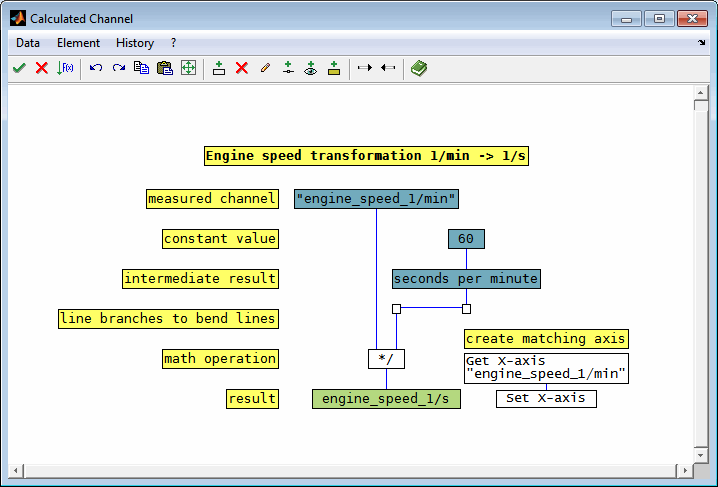
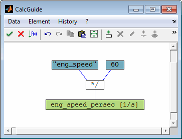
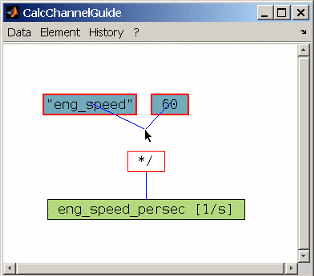
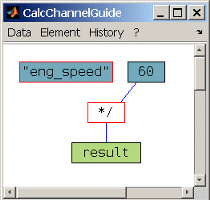
The following figure shows a very simple example to transform the engine speed input from unit 1/min to 1/s we need just four objects and three lines.
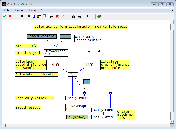
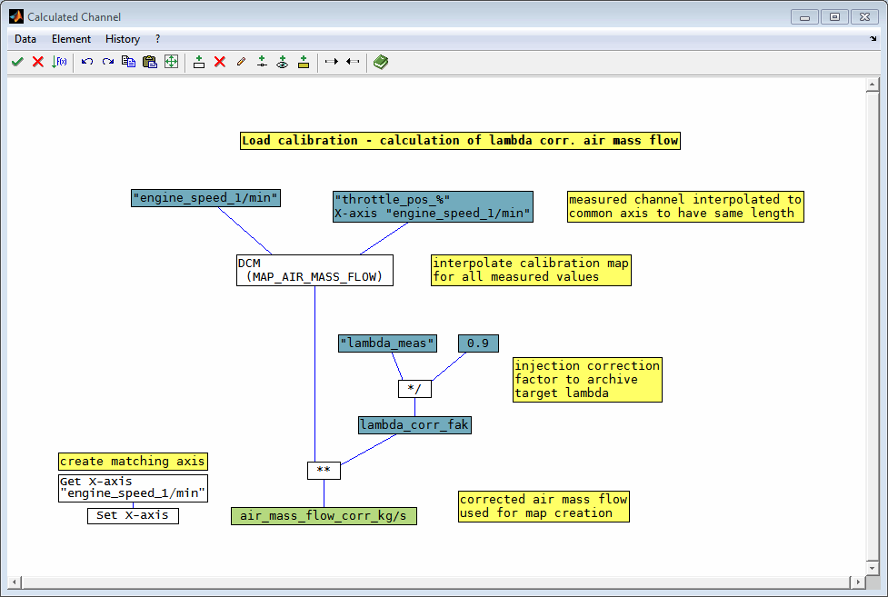
The next figure shows a more complex example to calculate a corrected load signal from a measured load and lambda signal and the lambda setpoint values that are interpolated from map in a calibration parameter file.
An adequate set of objects is available to realize all common calculations. Supported by comfortable assistant functions like history, file export/import, test and debugging features it is easy to realize complex calculations in a comprehensible manner.
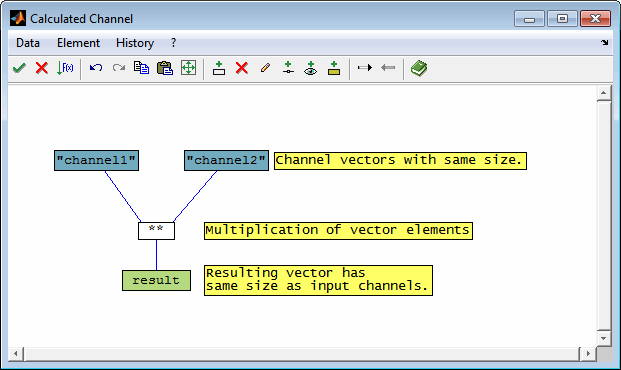
3.1 Vector based calculation strategy
By default calculations are performed vector based in a element wise manner. In the following example a multiplication of two vectors is implemented. This means that each element of “channel1” is multiplied with the element from “channel2” at the same position to retrieve the of the result at again the same position. Therefore both inport data vectors must have the same dimension and the resulting vector will also have this dimension.
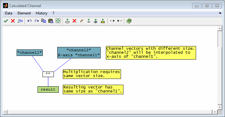
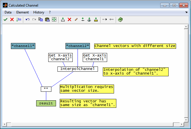
If data to combine in a calculation has different size its size usually needs to be adjusted. This can be done by interpolation. The following two figures show how to implement this. In the first one Channel2 is interpolated to the axis of Channel1 to adjust to its size using the “InterpolChannel” object. A convenient way to do this without additional objects is shown in the second figure. The “channel” objects provides an interpolation to an axis of another channel.
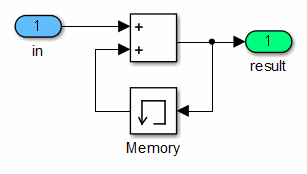
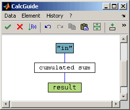
Since the calculations are done vector based there are objects available to implement fast calculations that are usually performed using loop constructions. As an example in the following figures the calculation of a cumulated sum is shown. The implementation in a simulation software on the left side has the same functionality as the one on the right side using the CalcGuide.
4 Help / Tutorials
A detailed help specific for each object is available when editing or double clicking a object. Each single input field of these dialog windows additionally has an individual help that can be opened by the “i” button or by using the F1 key when the field is activated.
A set of introduction documents and examples is available using the “?” menu item.
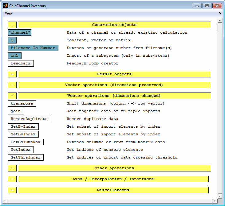
5 Objects
5.1 Types of objects
The objects available are structured in different groups. All objects are described in detail in the Object Inventory reference.
When you double click an object a configuration dialog will be shown. It starts with a short introduction to the objects and a port description followed by the configuration input fields if any. When an input fields is highlighted you can get a help dialog especially for that input fields by pressing “F1” or using the “i” button.
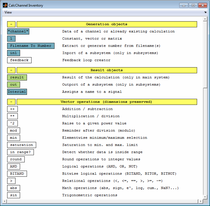
5.2 Generation objects
The calculation always starts from data from Generation Objects. Various generation objects are available. In addition to the definition of fixed values, they also allow access to dynamic data from outside.
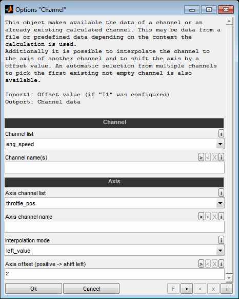
5.2.1 Channel object
With the channel object, for example, you can access measurement data or existing calculated channels. In order to access a previously calculated channel, it must be generated in the same pass and in the sequence before the second calculated channel. It is not possible to access calculated channels that already exist in the DataArtist, for example, but are not included in the current data loading process.
Additionally it is possible to interpolate the channel to the axis of another channel. This feature is used to adjust channel data to a common axis and therefore allows to perform direct operations like addition because the channels data will have same length after interpolation.
The axis of the channel may be shifted by a offset value. The offset will be applied before the interpolation to another axis if any. Positive values mean to shift the data to the "left" to smaller axis values. The offset can also result from an inport if “I1” is specified as offset value.
An automatic selection from multiple channels to pick the first existing not empty channel is also available. This feature eases to load data from channels with varying names - e.g. from different vehicles with different lambda measurement equipment installed. Keep in mind that the non existing channels may lead to harmless warnings during the calculation.
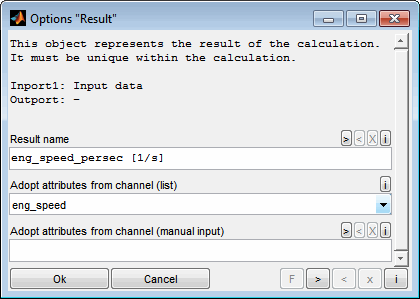
5.3 Result object
The result object has a special meaning. It represents the final result of the calculation. Each calculation must contain exactly one result object. Depending on the context of the calculation it may be possible to some object properties.
The name of the resulting calculated channel can be entered and a unit can be appended in [] brackets if supported by the calling application (e.g. DataArtist).
It is also possible to select a channel whose attributes will be transferred to the calculated channel. This allows for example the transfer of comments and value to text translations. The channel selected must already be in use inside the calculation (e.g. in a channel object). An automatic selection from multiple transfer channels to pick the first existing not empty channel is also available. This feature eases to handle data from channels with varying names - e.g. from different vehicles with different lambda measurement equipment installed. Keep in mind that the non existing channels may lead to harmless warnings during the calculation.
5.4 Add by symbol (Inventory)
The inventory (Shift+Ins, Space) shows all objects grouped and with their individual appearance. Additionally a short description is shown. The sections can be expanded and collapsed.
The inventory is opened by pressing the “space” key and the objects are added by double clicking them with the mouse or by their context menu. When a single line is selected before adding an object it will be inserted into the line automatically.
If the option is checked in the menu the inventory window will automatically hide when moving the mouse from it to the main figure window as long as both windows overlap.
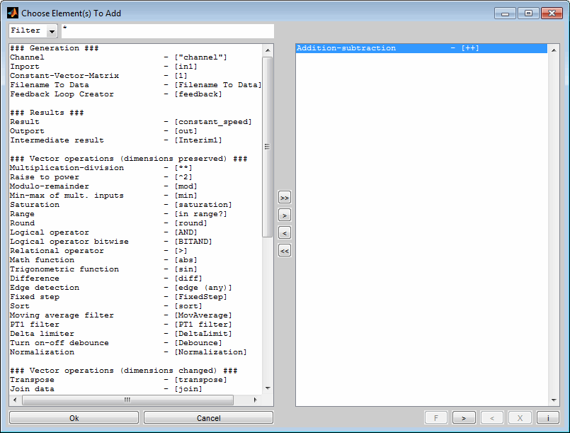
5.5 Add by name
The quick way to add objects is to add them by name (Ins). Just type “insert” to open the dialog. By typing letters and using the wildcard character * the view can be filtered. Select one or multiple objects to add.
When a single line is selected before adding an object it will be inserted into the line automatically.
6 Line connections
Lines are used to connect objects and to define the calculation order and the signal flow.
6.1 Object ports
Lines must be connected to inports and outports of objects. A line does always start at an outport of an object and must end at an inport of another object.
6.1.1 Inports
The number of inports depends on the type of objects and possibly on the configuration of the object. For example an constant does does not have any inports and the addition objects inports number depends on its configuration of the calculation signs. The introduction in the configuration dialog will give further information regarding the inports.
Only one line can be connected to an inport.
6.1.2 Outports
An object does only have exactly one or none outports.
Any number of lines can be connected to an outport. This way it is possible to split calculation paths.
6.2 Connecting objects
There are different methods to connect objects using lines.
Shift + Mouse drag
Draw a line from the source object to one of the target objects inports by dragging the mouse with the “Shift” key pressed.
Mouse click + wait + drag
Click with the mouse onto a object, wait a short time and move the mouse then to draw the line to a target objects inport. Without waiting you would have used the mouse to move the object.
Mouse double click
By double clicking to a point near the middle of the line intended to draw the nearest object with an available inport will be connected to the nearest object providing a outport.
In case of successful junction the objects connected will be colored green for a short time. In case no connection was created objects that were intended to be connected will be colored yellow for a short time. No connection will be created if only one suitable object was found or the double click mouse point was too far away from the connection line of the objects.
Move object over line
When moving a single object with the mouse and releasing it above a single line, the objects will be inserted into that line. The object must have an unconnected inport and outport for this to happen.
Add object with line selected
When a single line is selected before adding an new object it will be inserted into the line automatically.
Using the first two methods lines are drawn from all marked objects simultaneously. This way you can quickly connects multiple objects to one target objects.
If you draw just one line it will be connected to the nearest empty inport when you release the mouse button. The inports are horizontally distributed over the extent of the object. If you draw multiple lines at a time or when drawing lines by double click they will be connected starting from the left most yet not connected inport of the target object independent from where you release the mouse button. In case of connecting objects by double click the line will always be connected to the left most yet not connected inport.
If you release the mouse button outside any object or over an object without unconnected inports the line will be deleted.
When an object has multiple inports the number of the inport the line was connected to will be displayed shortly.
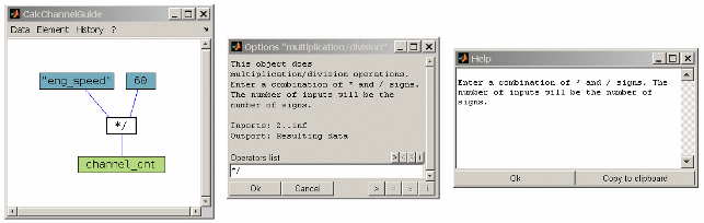
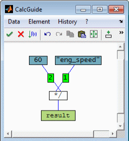
The horizontal order of the inports is important for some types of objects because inports are numbered from left to right and this order is used to insert them into the calculation. In the previous example the calculation to be done was defined as “*/”. So “eng_speed” must be connected to the left inport to be the numerator of the division. Hidden line crossings behind an object will influence the calculation order in a obscure way. Therefore they are detected and shown automatically. See section “Continuous plausibility check“ for further details.
6.3 Line branches
Line branches are used to bend lines (Double click line). This way it is possible to avoid line crossings and structure the calculation.
Additionally lines branches can be used to split calculation paths because multiple lines can be connected.
7 Editing / structuring the calculation
7.1 Copy objects
Objects can be copied and pasted by using the menu items or by just dragging them with the right mouse button (Ctrl + c, Ctrl + v). If multiple objects are marked all of them will be copied.
7.2 Move objects
Objects can be moved by dragging the with the mouse or using the arrow keys when they are marked.
When moving a single object with the mouse and releasing it above a single line, the objects will be inserted into that line. The object must have an unconnected inport and outport for this to happen.
7.3 Add comments
You can add comment objects to a calculation (Ctrl + Double click unused area). These are static text objects without inports and outports.
7.4 Fit window
Using the menu item or keyboard shortcut (Ctrl + f) you can quickly fit the window to the existing objects.
7.5 Unify fonts
It is possible to adjust all objects to a common font in case of import of objects from other computers with different fonts available.
7.6 Update objects
Newer software versions of the CalcGuide may include improvements, changes or bug fixes for the calculation of single objects. To apply these changes to all existing objects of a calculation an objects update can be performed. The update does apply to all objects except for subsystems. These must be updated separately.
After the update the number of updated objects will be shown.
8 Special objects
8.1 Configuration
This object is used to edit general setting of the calculation.
Perform test calculation
Use this option to activate or deactivate the test calculation. Before closing the CalcGuide window the calculation can be checked by performing a test calculation. The test calculation will be done using synthetic data. So the absolute values and dimensions cannot be judged and will not be shown. Visualization objects are not regarded when performing a test calculation if not explicitly enabled using the next option. The test calculation is usually much faster than the final calculation with the entire data.
Keep in mind that the synthetic inport data used may lead to irrelevant errors.
Process visualization objects during test calculation
Activate this option to enable visalization object during test calculation.
Runtime optimization (reduced checks)
Activate this option to minimize the runtime of the calculation. During the calculation, checks are performed to display meaningful messages in the event of a problem or error. These checks require a certain duration. If the calculation is used in a frequently recurring context, it may be useful to turn off these checks when the calculation functions reliably. This can reduce the duration of the calculation. In the event of problems, the checks can be reactivated at any time.
Waitbar delay
Some objects use a waitbar to indicate their calculation progress. The initial delay to show up the waitbar and the update cycle time can be edited. Increasing this value to avoid the waitbar showing up can improve the performance of frequently executed calculations significantly.
8.2 Subsystem
Subsystems are used to structure extensive calculations or to reuse parts of calculations as they can be copied easily.
Subsystems additionally have inport objects. These make available the data from the lines connected outside the subsystem. Similarly they have outports. Each subsystem must have exactly one outport object.
8.3 Axis objects
Objects to access and create x-axes inside the calculation are available.
Get X-axis
This object retrieves the x-axis of a channel from the file or an already existing calculated channel. The axis can be used inside the calculation or connected to an ''Add X-axis'' object to assign the x- axis for this calculated channel.
Set X-axis
This object is used to assign the X-axis of the calculated channel. If the dimension of the result of the calculation does not match exactly one existing x-axis you have to create an x-axis and assign it to be able to load the calculated data. This object is connected to the x-axis data and does the assignment. To assign an existing x-axis for this calculation use the "Get X-axis" object.
8.4 Simulink simulation
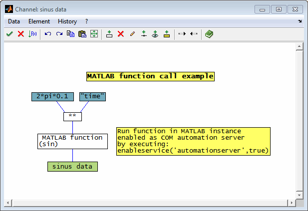
This object performs a Simulink simulation. Data exchange is done using MATLAB COM Automation server. The inport data of the object is first written to the MATLAB workspace. Then the simulation is started and after termination the output is retrieved from workspace or signal logging.
8.4.1 MATLAB COM automation server access
The connection is established to an existing MATLAB COM Automation server. Therefore a MATLAB instance must be running and COM Automation server must be activated. To do so use the following command:
enableservice('AutomationServer',true);
By default the connection is established to the most recent MATLAB version installed. If you want to connect to any MATLAB version other than the most recent one installed you need to enter the correct version string (available from MATLAB command “version”) in the object options.
8.4.2 Simulink model configuration
Signal / parameter access
To access signals and parameters for setting them to values produced by CalcGuide and to retrieve the simulation result the MATLAB workspace is used. The object supports to write the inport data to the MATLAB base workspace and to retrieve the simulation output and simulation time from it.
The workspace variables assigned by the CalcGuide can then be used to configure the Simulink blocks or feed inports – e.g. by using “From Workspace” and “To Workspace” blocks or by writing the variable names to the corresponding parameter configuration fields of the system or blocks. Alternatively a Simulink simulation can retrieve its input data and time from workspace variables directly using the “Load from workspace” feature from the model configuration.
“From Workspace” block
This block reads data values from the MATLAB workspace. For matrix formats as provided from the CalcGuide, at least two columns must exist. The first column contains the time vector and the subsequent columns are data values. Creating the matrix can be done directly in the corresponding input field.
Example:
[axis eng_speed] : Build matrix from two workspace vectors “axis” and “eng_speed” assigned by the CalcGuide.
[(1:length(eng_speed))' eng_speed] : Build matrix from workspace vector “eng_speed” assigned by the CalcGuide and add an axis starting from 1 with increment 1.
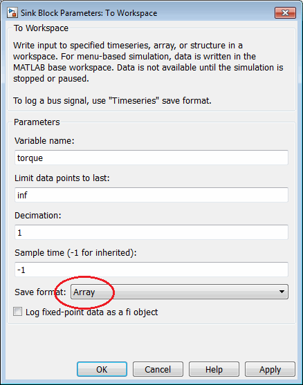
“To Workspace” block
This block writes data values to the MATLAB workspace. It is important to use the “Array” save format for the CalcGuide to access the data. The data must be a vector or matrix. If you want to retrieve multiple signals from a simulation you may create a matrix in Simulink with one signal per column and in CalcGuide you can extract the columns using the “GetColumnRow” object. To create a matrix in Simulink from multiple signals with equal length use a bus creator.
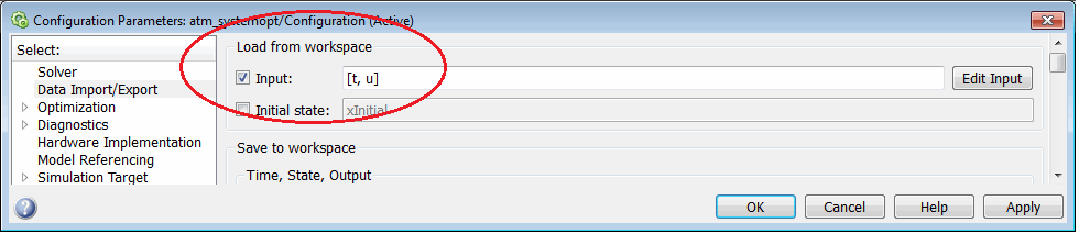
“Load from workspace” configuration
A Simulink simulation can retrieve its input data and time from workspace variables directly using the “Load from workspace” feature from the model configuration. To do this, you must join as many signals in the CalcGuide as the Simulink system has inputs in row direction to a matrix using a "join" object. Additionally the simulation time vector must be passed.
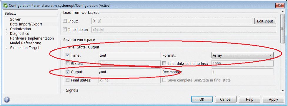
“Save to workspace” configuration, Simulation time output
To access the Simulink simulation output and time in CalcGuide you can use the Model Configuration dialog in Simulink to export it to workspace. The configuration of the CalcGuide object the enables to retrieve the time and append it to the simulation output data. Therefore you must ensure that the length of the simulation time will be the same as the length of the simulation output data. See “Simulink simulation object configuration” for details.
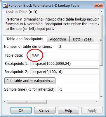
Block parameters
Block parameters can be filled directly from the workspace variables. In the example below the lookup table values are retrieved from workspace. They will be assigned by CalcGuide and result from DCM objects in the CalcGuide calculation.
Changed conventions for the dimensions must be observed. While in the SGE Circus, the x-axis is the horizontal axis of a map, in MATLAB/Simulink, for example, it is the vertical axis. Therefore, for direct use of the output of a DCM object as a Simulink block parameter, it is necessary to transpose. This is easy to achieve because it is an option of the DCM object.
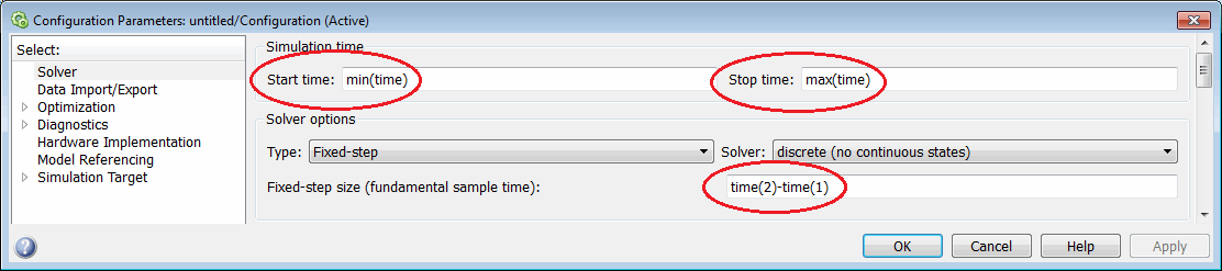
Simulation solver / time
The simulation behavior will be determined by the settings chosen in Simulink. The resulting data to return from MATLAB workspace to CalcGuide results from this settings. So the solver and simulation time settings give the size of the resulting data. If the timing is relevant you need to ensure the correct behavior through the Simulink model configuration and by passing time from CalcGuide to the simulation – e.g. by additionally passing the (time) axis vector of an inport channel and using it to fill the corresponding parameters of the model configuration. See the following figure for an example.
If you need to ensure a given length of the resulting simulation data and time usually a discrete step solver with fixed step size must be used. The fixed step size may also be calculated from a workspace axis passed by CalcGuide.
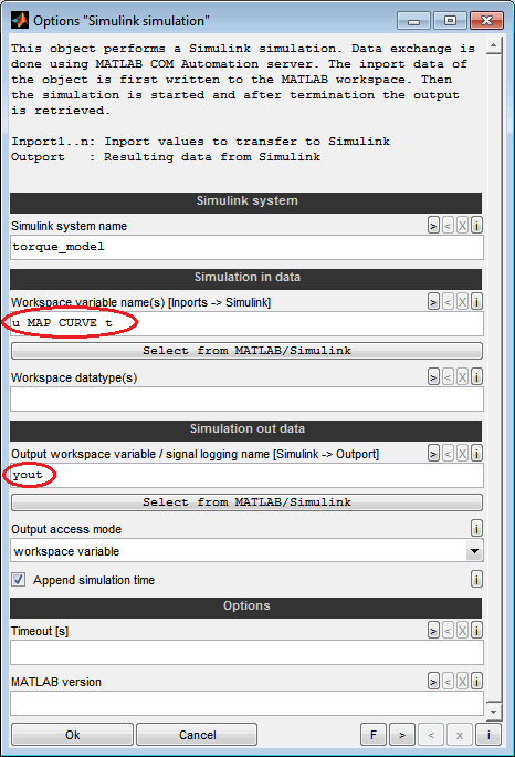
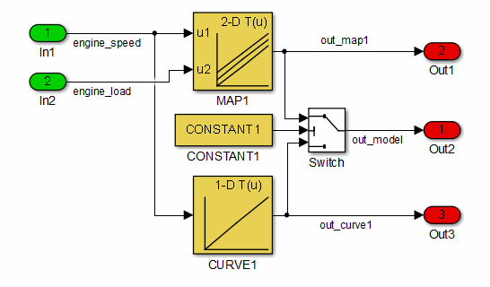
8.4.3 Simulink simulation object configuration
In the following figures a simple calculation is show as well as the configuration dialog of the object. The calculation feeds the Simulink system with some signals from measured channels, a time axis and two calibration parameters. The output of the simulation is retrieved, split into time and data and written to the calculation outport data.
The example is shown for data transfer using “From/To workspace” blocks in Simulink as well as for using the Simulink “Load from / Save to workspace” feature.
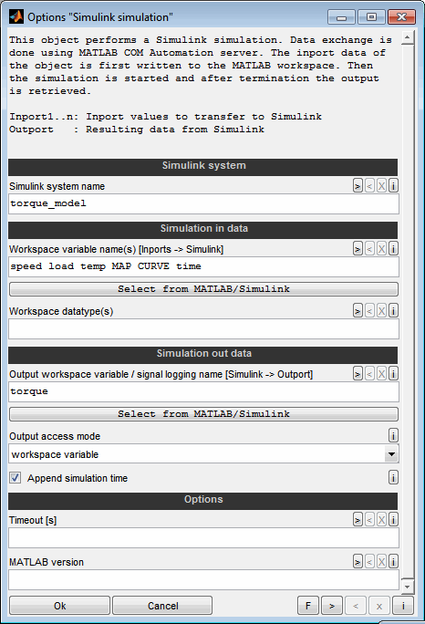
Simulink system name
Enter the name of the Simulink system to use. Leave empty to use the most recent opened system. Fill to use a specific system. Using a system on the MATLAB search path without opening it will result in a performance improvement. You need to enter the exact name from the system window title or returned by "bdroot" command. Do not enter e.g. the filename.
Workspace variable name(s) [Inports -> Simulink]
Enter a space separated list of workspace variable names to write the inport data of the object to. The inport data will be written to the MATLAB workspace before simulation start. The workspace variables can be used to configure Simulink objects or feed inports e.g. by using "From Workspace" blocks or by writing the variable names to the corresponding parameter configuration fields of the system or blocks. Alternatively a Simulink simulation can retrieve its input data and time from workspace variables directly using the “Load from workspace” feature from the model configuration. Therefor the single signals must be joined to a matrix in CalcGuide.
The names must be valid MATLAB variable names. A valid variable name starts with a letter followed by letters, digits or underscores. The data will be written to the MATLAB base workspace. The number of signal names gives the number of inports of the object. The workspace data can be used to feed the simulation with input data or the parameterize Simulink blocks.
The following pushbutton allows a comfortable selection from a list of all current MATLAB workspace variables. To do this, MATLAB must be started and activated as an AutomationServer by executing "enableservice(''AutomationServer'',true)".
Changed conventions for the dimensions must be observed. While in the SGE Circus, the x-axis is the horizontal axis of a map, in MATLAB/Simulink, for example, it is the vertical axis. Therefore, for direct use of the output of a DCM object in Simulink, it is necessary to transpose. This is easy to achieve because it is an option of the DCM object.
Example for three inports:
in1 in2 in3
Workspace data type(s)
Enter a space separated list of datatypes of the workspace variables to set. List must have same length as "Workspace variable name(s)". Valid data types are "double", "single", "uint8", "int8", "uint16", "int16", "uint32", "int32" and "logical". The data types must agree with the ones of the signals/variables in Simulink. You do not need to worry about the data types of the inport data. The conversion to the suitable datatypes is done automatically.
Leave empty to keep the datatypes of the inport data and enter only one entry to use for all inputs. "double", "single" and "logical" can be shortened to "d", "s" and "l".
Examples:
double double logical
single
d d s uint8
Output workspace variable / signal logging name [Simulink -> Outport]
Enter a space separated list of names of a workspace variables or signal logging elements to retrieve the outport data of the object from. To access a workspace variable a “To Workspace” block must be used or the Simulink model configuration must be set to save the data to the workspace, e.g. to the variable “yout”. To access a signal logging elements the Simulink model configuration must be set to save the signal logging data to a workspace variable named “logsout” in format “Dataset”. In case multiple elements are requested the output of the objects will be a matrix where each column represents one element. Therefore all elements to retrieve must be vectors with equal length.
The following pushbutton allows a comfortable selection from a list of all current MATLAB workspace variables / signal logging elements. To do this, MATLAB must be started and activated as an AutomationServer by executing "enableservice(''AutomationServer'',true)" and the Simulink model must be opened or in the MATLAB search path.
Example:
out1
out1 out2
Output access mode
The simulation output can be retrieved from a workspace variable or from a signal logging element. Select which access mode to use.
Append simulation time
When this option is used the simulation time vector will be retrieved in addition to the data from the "Output workspace variable / signal logging name" entered above. Both vectors must have same length and will be concatenated to a matrix to build the outport data of the object. The first columns will be the data vector(s) and the last column will be the time. In case the simulation data is already a matrix its row number must match the simulation time length to be able to append the time as last column. Use a "GetColumnRow" object to extract the single parts.
In case the simulation output is retrieved using a workspace variable the time must also be available in a workspace variable named “tout”. Set the Simulink model configuration to save the simulation time to a workspace variable. In case of accessing a signal logging element the simulation time will be detected automatically and must not be saved to workspace.
Timeout [s]
Enter a timeout value for the simulation in seconds. Use this option to avoid a blocking calculation in case the Simulink system has infinite stop time or does not terminate for any other reason. In case a lock happens you may kill the MATLAB process to proceed at least the calculated channel. Must be empty or a scalar timeout value in seconds >= 0.
MATLAB version
Enter the version string of the MATLAB version to connect to. This option is only needed if multiple MATLAB versions are installed on the computer and you want to connect any version instead of the most recent one. The connection will be established to a running MATLAB Automation server. This is a running MATLAB instance when "enableservice(''AutomationServer'',true)" was executed. In case multiple MATLAB versions are installed on the computer the connection will always be established to the most recent version of MATLAB by default. If you need to connect to a older version you need to enter the version string here. You can retrieve it by executing "version" in MATLAB.
Example:
8.2.0.701 (R2013b)
8.5 Simulink Host-Based Shared Library (*.dll)
This object computes the output of a Simulink Host-Based Shared Library (*.dll). Simulink systems can be included in CalcGuide calculation when they are compiled to a Host-Based Shared Library (*.dll). Therefore the build target must be set to "ert_shrlib.tlc".
It is possible to access signals and parameters to set them to values produced by CalcGuide and to retrieve the simulation result. The library calculation is done in a loop for every simulation step. After setting the entire values of “parameter” inports the proceeding for every simulation step is:
Set values of “signal” inports to the actual index value of the connected data.
Calculate library simulation step.
Retrieve library output values and write to actual index of the object outport data.
If the timing is relevant you need to ensure the correct behavior through the Simulink model configuration or by passing time from CalcGuide to the library – e.g. by additionally passing the (time) axis of an of an inport channel and using it within the system.
8.5.1 Simulink model configuration
To access signals and parameters of the system with the inports and the outport of the “Simulink DLL” object and to ensure correct library functionality some conditions must be kept.
Model Configuration parameters
Build target must be “ert_shrlib.tlc”.
A fixed step solver must be used. Set the “Tasking mode for periodic sample times” setting to “SingleTasking”.
“Single output/update function” setting must be activated.
Set the storage class of all signals and workspace variables to access to “ExportedGlobal” (see below for details).
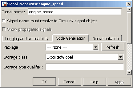
Signal access
Signals to access must have a name and their storage class must be set to “ExportedGlobal”. See the following screenshot of the signal properties dialog for an example configuration of a signal. The data type of a signal is also important for the configuration later on in CalcGuide. Is is determined by the blocks the signal arises.
Parameter access
Parameters are usually workspace variables in Matlab that are used to fill lookup tables, their axes and constant scalar source blocks with data or to parameterize other blocks. These parameters can be scalar values, vectors, matrices, grids of higher dimensions or even structures.
Parameters to access must also have their storage class set to “ExportedGlobal”. This can be done using the “Model Configuration Parameters” dialog to access the list of workspace variables. In the following figures this dialog is shown as well as the block parameters dialog to set the workspace variable name.
Changed conventions for the dimensions must be observed. While in the SGE Circus, the x-axis is the horizontal axis of a map, in MATLAB/Simulink, for example, it is the vertical axis. Therefore, for direct use of the output of a DCM object as a Simulink block parameter, it is necessary to transpose. This is easy to achieve because it is an option of the DCM object.
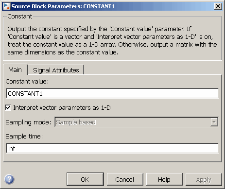
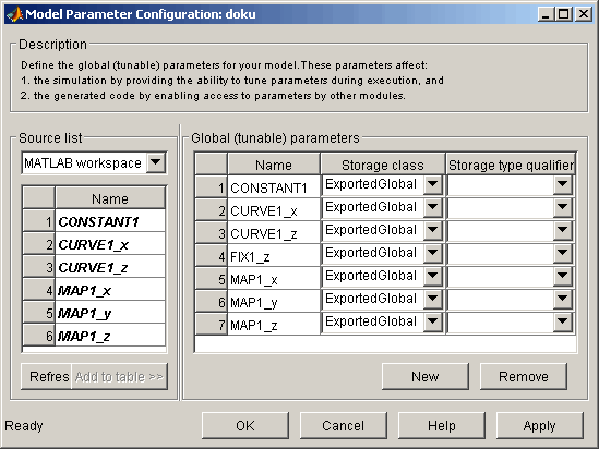
Before building the library fill all referenced parameter variables must exist in the workspace. The size of these variables is important for their access from the CalcGuide. Also their datatype is important and is defined in the block parameters.
8.5.2 Simulink DLL object
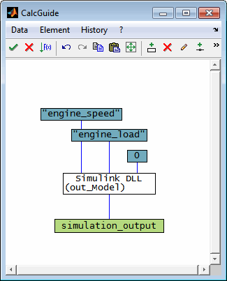
When the library was generated it can be used from “Simulink DLL” object in the CalcGuide. In the following figures a simple calculation is show as well as the configuration dialog of the DLL object. The calculation feeds the library with two signals from measured channels and a constant value. The output of the library is directly written to the calculation outport data. It is supported to retrieve multiple outputs as once. In case multiple outputs are retrieved they are concatenated to a matrix where each column is a signal.
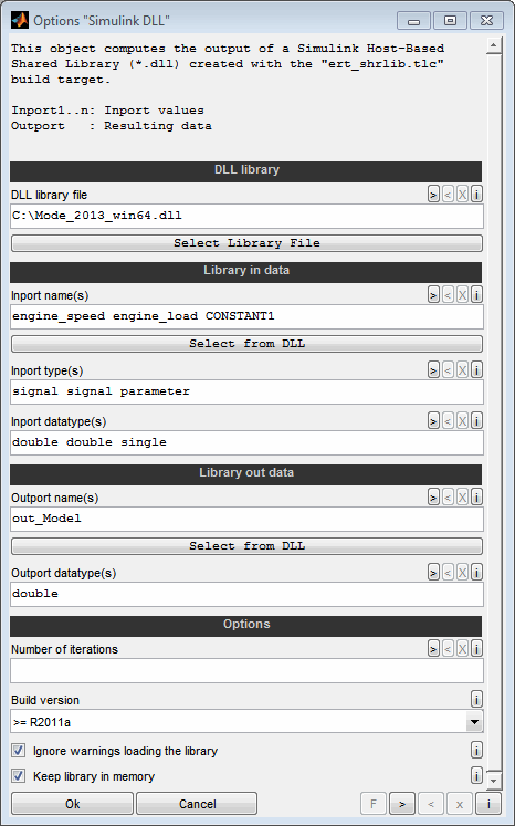
DLL library file
Enter the filename incl. path of the Simulink Host-Based Shared Library to use (*.dll). The file can be created in Simulink using the "ert_shrlib.tlc" build target. Leave empty to ask after confirming this dialog or use the following pushbutton to fill this field. Insert "**ask**" or "**ask_once**" to ask the user each time the channel is calculated. In case of "**ask_once**" all objects will share the same file.
The library must be build for the architecture of the SGE_Circus (32bit/64bit). Make sure to not rename the DLL file generated from Simulink. Otherwise the methods for initialization and step function cannot be determined. All required header files must be present in the same location. Also it might be necessary to provide a so called MATLAB prototype file. To properly load the library in case of a 64bit architecture additionally a so called thunk file is required.
The thunk and prototype file must match a certain naming and can be created in Matlab with the following command:
loadlibrary('<libraryfile>.dll','<headerfile>.h','mfilename','<libraryfile>');
<headerfile> (without ending) must be different from <libraryfile> (without ending) for this command to work properly. Rename the header file if necessary. The workspace variables referenced in the model must be present for this command to work properly.
Regarding the file name the following rule applies. Assuming that the library is named "<library>_win/32/64.dll":
→ 64bit thunk file: "<libraryfile>_thunk_pcwin64.dll"
→ Prototype file: "<libraryfile>.m"
When you select the library file from the object configuration dialog the process of copying the header files and generating the prototype and thunk is assisted automatically.
When a calculation includes other DLL objects referencing the same previous file you will be asked whether to transfer the file name to the other objects. This may be done only for the actual or all calculations.
Inport name(s)
Enter a space separated list of names of the inports. The names must exactly match the names of the referenced signals/variables in the Simulink system or workspace. These can be scalar values, vectors matrices or even structures. A special object is available to create a structure in the CalcGuide. Consult the header file related to the library used to obtained the correct names.
Signals or variables to access must have storage class "ExportedGlobal" in the Simulink system.
The following pushbutton allows a comfortable selection from a list of all signals/variables declared as ''ExportedGlobal'' in the Simulink system and the corresponding header file.
Changed conventions for the dimensions must be observed. While in the SGE Circus, the x-axis is the horizontal axis of a map, in MATLAB/Simulink, for example, it is the vertical axis. Therefore, for direct use of the output of a DCM object as a Simulink block parameter, it is necessary to transpose. This is easy to achieve because it is an option of the DCM object.
Example for three inports:
engine_speed engine_load CONSTANT1
Inport type(s)
Enter a space separated list of types of the inports. Valid types are "signal" and "parameter".'
"signal":
This typically means a Simulink signal connected to a inport block. In every calculation step all inports of type "signal" will be set to the actual index value of the data connected to it. Therefore "signal" inports will be fed dynamically with single values of the inport data which also means that for all "signal" inports the connected data must be vectors of same length.
'"parameter:"
These library inputs are always fed with the entire connected data. Typically "parameter" inputs are workspace variables in Simulink that are used to fill lookup tables, their axes, constant scalar source blocks or parameters of other blocks. These can be scalar values, vectors matrices or even structures. A special object is available to create a structure in the CalcGuide.
Thus it is essentially important that the connected data size matches the size of the Simulink data. Otherwise unpredictable behavior may occur including software crashes. The required size can be obtained from the Simulink system or the header file related to the library file used.
The list must have same length as "Inport name(s)". Leave empty to set all types to "signal".
Example for three inports:
signal signal parameter
Inport datatype(s)
Enter a space separated list of datatypes of the inports in the library. List must have same length as "Inport name(s)". Valid data types are "double", "single", "uint8", "int8", "uint16", "int16", "uint32", "int32" and "logical" and any type known to the library. Unlike other objects the datatype strings cannot be shortened.
The data types must agree with the ones of the signals/variables in Simulink. For structure arguments consult the header file related to the library used to obtained the correct data type term. The terms in the header file may differ from the workspace name. E.g. for structures the term may be something like “struct_NPeESu6laOazJ7L91w1w3G”. For structure datatypes it is mandatory to have a MATLAB prototype file present with the library. The file must match a certain naming and can be created in Matlab with the following command:
loadlibrary('<libraryfile>.dll','<headerfile>.h','mfilename','<libraryfile>');
You do not need to worry about the data types itself of the inport data connected to the inports. The conversion to the suitable datatypes for the library is done automatically.
Leave empty to keep the datatypes of the inport data and enter only one entry to use for all inputs.
Example for four inports with the last one being a structure:
double double logical struct_NPeESu6laOazJ7L91w1w3G
Outport name(s)
Enter a space separated list of names of the outports to retrieve. The names must exactly match the names of the referenced signal/variable in the Simulink system. It must be a scalar value - usually a Simulink signal. In case multiple outports are requested the output of the objects will be a matrix where each column represents a signal.
Signals or variables to access must have storage class "ExportedGlobal" in the Simulink system.
The following pushbutton allows a comfortable selection from a list of all signals/variables declared as ''ExportedGlobal'' in the Simulink system and the corresponding header file.
Example:
out1
out1 out2
Outport datatype(s)
Enter a space separated list of datatypes of the outports. List must have same length as "Outport name(s)". Valid data types are "double", "single", "uint8", "int8", "uint16", "int16", "uint32", "int32" and "logical". The datatypes must agree with the ones of the signal/variable in Simulink.
Number of iterations
Using this option you can force a definite number of simulation steps to execute. This option is needed when no “signal” inports are available to retrieve the simulation step number from. Leave empty to determine the step number from the inport length of "signal" inports.
Build version
Select the version of the software build.
Ignore warnings loading the library
When enabling this option you will receive no warnings when the library is loaded. This is usually used to ignore warnings about missing symbols that do not affect the calculation.
Keep library in memory
If this option is enabled, the library will be loaded into memory and reused. The repeated execution of the calculation is thus faster. Changes to the library file are ignored. If this option is not active, the library is reloaded each time the calculation is executed.
8.6 MATLAB function / mex
This object integrates a MATLAB function or mex call into a calculation. In this way, you can integrate internal MATLAB functions, custom functions, and even C code. Data exchange is done using MATLAB COM Automation server. The inport data of the object is first transferred to MATLAB. Then the function call is evaluated in MATLAB and termination the output is retrieved.
8.6.1 MATLAB COM automation server access
The connection is established to an existing MATLAB COM Automation server. Therefore a MATLAB instance must be running and COM Automation server must be activated. To do so use the following command:
enableservice('AutomationServer',true);
By default the connection is established to the most recent MATLAB version installed. If you want to connect to any MATLAB version other than the most recent one installed you need to enter the correct version string (available from MATLAB command “version”) in the object options.
8.6.2 MATLAB object configuration
Signal / parameter access
To access signals and parameters for setting them to values produced by CalcGuide and to retrieve the function result you can use either the MATLAB workspace or the function input and output parameters.
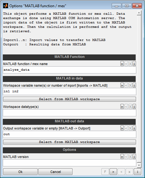
MATLAB function / mex name
Enter the name of the MATLAB function or the mex function to call. Make sure that the function is on the MATLAB search path. You need to enter the exact name of the function. Do not enter e.g. the filename.
Workspace variable name(s) or number of inport [Inports -> MATLAB]
Input data can be transferred to MATLAB in two ways. Either they are written to the workspace or directly to the function to be called as a parameter.
If the parameters are to be written to the workspace enter a space separated list of workspace variable names to write the inport data of the object to. The workspace variables can then be used inside the MATLAB function. The following pushbutton allows a comfortable selection from a list of the currently available MATLAB workspace variables. To do this, MATLAB must be started and activated as an AutomationServer by executing "enableservice(''AutomationServer'',true)".
If the parameters are to be passed directly to the function, enter the number of inports. In this case, all connected inport signals are transferred to the function as parameters in the sequence they are connected.
The names must be valid MATLAB variable names. A valid variable name starts with a letter followed by letters, digits or underscores. The data will be written to the MATLAB base workspace. The number of signal names gives the number of inports of the object.
Example for three inports to workspace:
in1 in2 in3
Example for three inports passed as parameters:
3
Workspace datatype(s)
Enter a space separated list of datatypes of the workspace variables to set. List must have same length as "Workspace variable name(s)". Valid data types are "double", "single", "uint8", "int8", "uint16", "int16", "uint32", "int32" and "logical". The data types must agree with the ones of the signals/variables in Simulink. You do not need to worry about the data types of the inport data. The conversion to the suitable datatypes is done automatically.
Leave empty to keep the datatypes of the inport data and enter only one entry to use for all inputs. "double", "single" and "logical" can be shortened to "d", "s" and "l".
Examples:
double double logical
single
d d s uint8
Output workspace variable or empty [MATLAB -> Outport]
Enter a space separated list of workspace variables to retrieve the outport data for or leave empty to use the first function return value. The following pushbutton allows a comfortable selection from a list of the currently available MATLAB workspace variables. To do this, MATLAB must be started and activated as an AutomationServer by executing "enableservice(''AutomationServer'',true)".
In case multiple elements are requested the output of the objects will be a matrix where each column represents one element. Therefore all elements to retrieve must be vectors with equal length.
Example:
out1
out1 out2
MATLAB version
Enter the version string of the MATLAB version to connect to. This option is only needed if multiple MATLAB versions are installed on the computer and you want to connect any version instead of the most recent one. The connection will be established to a running MATLAB Automation server. This is a running MATLAB instance when "enableservice(''AutomationServer'',true)" was executed. In case multiple MATLAB versions are installed on the computer the connection will always be established to the most recent version of MATLAB by default. If you need to connect to a older version you need to enter the version string here. You can retrieve it by executing "version" in MATLAB.
Example:
8.2.0.701 (R2013b)
8.7 For loop subsystem
For loop subsystems can be used to implement iterative calculations. Remember that by default all calculations are performed vector based in one step. So for example to calculate a cumulated sum there is no need to use a for loop subsystem – see section ”Vector based calculation strategy“ for details.
For loop subsystems have three additional inports for the start, increment and final value of the loop counter. Inside the subsystem a LoopIndex object is available to access the loop counter. As an example the following figures show the outer and inner view of a for loop subsystem used to set the first ten values of the engine speed data to NaN.
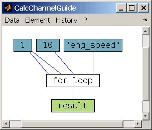
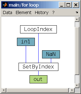
Implementing calculations in for loops requires to understand how they are implemented. Before the first run of a for loop subsystem the inports are initialized with the data from the outer system and the LoopIndex is initialized with the value from the first inport. During the run the LoopIndex will be incremented before each loop with the seconds inport value and the calculation is performed. This proceeding is repeated as long as the LoopIndex is <= the third inports value.
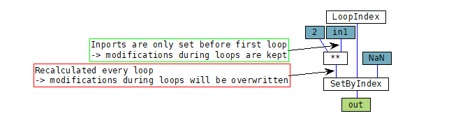
So if you intent to modify data e.g. using the SetByIndex object it only makes sense to modify data directly resulting from an inport object because this data is initialized before the first loop and not modified afterwards by the loop calculation. Data downstream the calculation is not suitable for modification because it will be overwritten every loop. The following faulty example is similar to the previous one but additionally meant to multiply the result by two. In this case the SetByIndex object will modify data that will be overwritten every loop by the multiplication and so the modification will get lost.
Be aware that loop calculations may last very long. Prefer elementwise operations if available for the intended task. A for loop will show up a waitbar if it is executed.
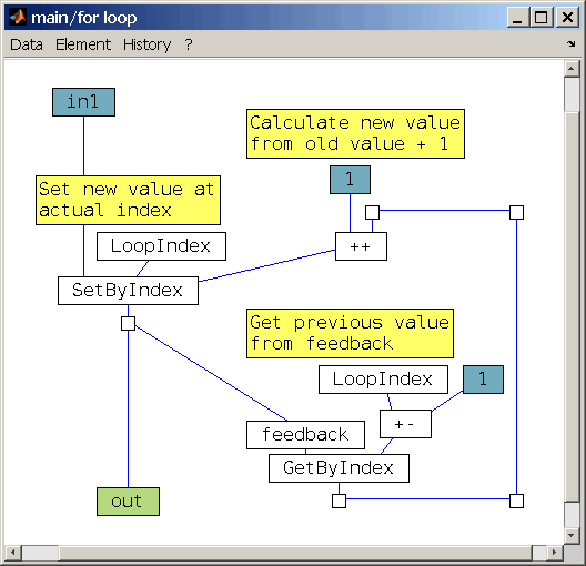
8.8 Feedback creator
This object is used to create a feedback loop. Connected to an outport it allows to use this signal ahead in the calculation. This is mainly useful inside loops to repetitively calculate values depending on their previous value.
Remember that by default all calculations are performed vector based in one step. So for example to calculate a cumulated sum there is no need to use a feedback object in a loop subsystem – see section ”Vector based calculation strategy“ for details.
The initial value of the outport of a feedback object can be specified. Remember to specify the initial value to be a vector of adequate length if the initial loop index is greater than 1.
The following example implements a calculation to create a vector containing increasing values from 1 to 100.
9 Debugging
9.1 Continuous plausibility check
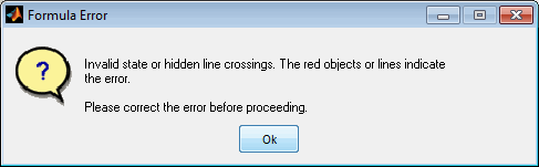
During editing the calculation a continuous plausibility check is done. Objects that have an inconsistent state are marked with a red border color. This will happen for example if not all necessary ports are connected or if a object that must be unique is inserted multiple times.
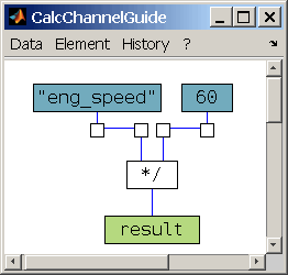
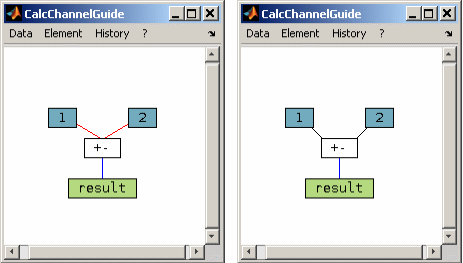
Inport lines of a object will be marked with red color if they cross each other behind the object (hidden line crossings). This is usually caused by a messed connection order of the lines from left to right and may lead to unexpected calculation results. In the following figure on the left side the constant “1” is connected to the right inport of the subtraction and the constant “2” is connected to the left inport. Therefore the calculation result would be 1 instead of -1 like in the figure on the right side with the constants connected correctly.
9.2 Visualization
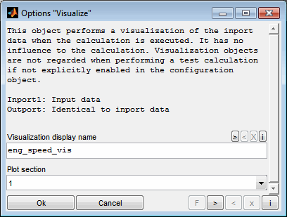
It is possible to visualize part of the intermediate calculation results. You can add any number of visualization objects. This is done by double clicking a line with the “Control” button pressed (Ctrl + Double click line). When the calculation is performed each visualization objects produces a graphical (for vectors) or numeric (for scalars) output. Visualization objects are not regarded when performing a test calculation if not explicitly enabled using the configuration object.
For a visualization object the name to display in the corresponding legend entry of the graphics and the plot section can be configured. The legend entry will also indicate the size of the data displayed. If you spread your visualization objects over multiple plot sections the visualization window will be split into separate axes sections. A plot section can contain one or multiple visualization object outputs.
In the visualization window you can use for example the zoom and data cursor functionality to analyze the calculation data.
9.3 Test calculation
Before closing the CalcGuide window the calculation can be checked by performing a test calculation (Ctrl + t). The test calculation will be done using synthetic data. So the absolute values and dimensions cannot be judged and will not be shown. Visualization objects are not regarded when performing a test calculation if not explicitly enabled using the configuration object. The test calculation is usually much faster than the final calculation with the entire data.
The test calculation is done by default when confirming the calculation. This can be turned off using the configuration object.
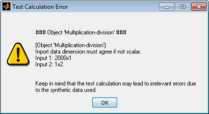
Keep in mind that the synthetic inport data used may lead to irrelevant errors. If the test calculation results in an error, this does not necessarily mean that there is something wrong with the calculation, it is only an indication.
9.3.1 Inports number display
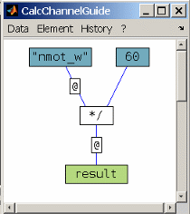
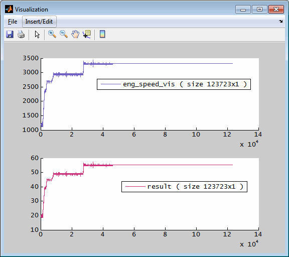
In a first step all lines connected to objects with at least two inports are numbered. This helps to judge the calculation order of the inport signals. In the following example we can see that the channel “eng_speed” is used as the numerator of the division because it is connected to inport 1.
9.3.2 Error indication
The result of the test calculation will be displayed by colored highlighting of the objects. Successfully processed objects will be shown with green border color and objects causing a calculation error will be shown with red border color. Unprocessed objects keep their border color. If an error occurs a corresponding message will be shown.
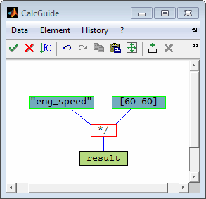
In the following example the error is caused by trying to divide two vectors with different dimensions.
But keep in mind that due to the synthetic data and data dimensions errors may occur that will not occur when the calculation is performed using the real data. For example the synthetic data used for a division may contain a zero and lead to an error while the real data does not contain zeros and the calculation will run fine.
9.3.3 Unprocessed objects indication
When the calculation is composed usually all objects should take place. In case there remain unprocessed objects a corresponding message will be shown and the objects will be shown with red border color.
A typical case leading to unprocessed objects is to create calculation loops without integrating a feedback object – see the following example.
9.3.4 Hidden line crossing indication
The result of the test calculation will be displayed by colored highlighting of the objects. Successfully processed objects will be shown with green border color and objects causing a calculation error will be shown with red border color. Unprocessed objects keep their border color. If an error occurs a corresponding message will be shown.
In the following example the error is caused by trying to divide two vectors with different dimensions.
But keep in mind that du
10 History
10.1 Save to file / load from file
The actual calculation objects can be exported to a file (Ctrl + s) and also be filled from a file (Ctrl + o). As also this functionality is available via shortcuts it is very easy to keep records of the work done and also to redo some work by reusing calculations or calculation parts. Not only the loading of files exported from CalcGuide is supported. It is also possible to load from files saved elsewhere that contain calculations – e.g. during loading data in DataArtist.
When exporting with some objects marked you will be asked whether you want to export all or only the marked objects. When importing from a file with already some objects existing you will be asked if you want to add the new objects or replace the existing ones.
11 Object inventory reference
11.1 Generation objects
channel
This object makes available the data of a channel or an already existing calculated channel. This may be data from a file or predefined data depending on the context the calculation is used. The channel must already exist or be a previously calculated channel. In order to access a previously calculated channel, it must be generated in the same pass and in the sequence before. It is not possible to access computer channels that already exist in the DataArtist, for example, but are not included in the current data loading process.
Additionally it is possible to interpolate the channel to the axis of another channel. This feature is used to adjust channel data to a common axis and therefore allows to perform direct operations like addition because the channels data will have same length after interpolation.
The axis of the channel may be shifted by a offset value. The offset will be applied before the interpolation to another axis if any. Positive values mean to shift the data to the "left" to smaller axis values. The offset can also result from an inport if “I1” is specified as offset value.
An automatic selection from multiple channels to pick the first existing not empty channel is also available. This feature eases to load data from channels with varying names - e.g. from different vehicles with different lambda measurement equipment installed. Keep in mind that the non existing channels may lead to harmless warnings during the calculation.
Inport1: Offset value (if "I1" was configured)
Outport: Channel data
constant/vector/matrix
This object generates a constant, vector or matrix. The dimension can be fix or depend on inports values. See the input field help for further details.
Inports: -
Outport: Constant data
Filename To Data
This object enables to extract or generate numbers from the names of the files that deliver the data. Use to affect the calculation depending on the files. For example you can extract the engine speed from the filename or a number characterizing the hardware configuration.
Inports: -
Outport: Number from filename(s)
inport
This object represents an inport of a subsystem. A subsystem may contain an arbitrary number of inports. Outside the subsystem all inports must be connected. The number to assign to the inport can be modified. The actual number of the modified inport will be swapped with the inport owning the new number.
Inports: -
Outport: Data connected outside the subsystem.
From MATLAB
This object retrieves a numeric MATLAB workspace variable. Data exchange is done using MATLAB COM Automation server.
Inports: -
Outport: Resulting data from MATLAB.
feedback
This object is used to create a feedback loop. Connected to an outport it allows to use this signal ahead in the calculation. The initial value can be specified. Remember to specify the initial value to be a vector of adequate length if the initial loop index is greater than 1.
Remember that by default all calculations are performed vector based in one step. So for example to calculate a cumulated sum there is no need to use a feedback object in a loop subsystem – see section ”Vector based calculation strategy“ for details.
Inport1: Input data
Outport: Feedback data
11.2 Result objects
result
This object represents the result of the calculation. It must be unique within the calculation. The name of the resulting calculated channel can be entered and a unit can be appended in [] brackets if supported by the calling application (e.g. DataArtist).
It is also possible to select a channel whose attributes will be transferred to the calculated channel. This allows for example the transfer of comments and value to text translations. An automatic selection from multiple transfer channels to pick the first existing not empty channel is also available. This feature eases to handle data from channels with varying names - e.g. from different vehicles with different lambda measurement equipment installed. Keep in mind that the non existing channels may lead to harmless warnings during the calculation.
Inport1: Input data
Outport: -
outport
This object represents an outport of a subsystem. A subsystem may contain an arbitrary number of outports. Outside the subsystem all outports must be connected.
Inport1: Input data
Outport: -
intermediate result
This object is used to assign a name to a signal. It has no influence to the calculation.
Inport1: Input data
Outport: Identical to inport data
11.3 Multiple vector operations (dimensions preserved)
addition/subtraction
This object does addition/subtraction operations. Enter a combination of + and - signs. The number of inputs will be the number of signs.
Inports: 2..inf
Outport: Resulting data
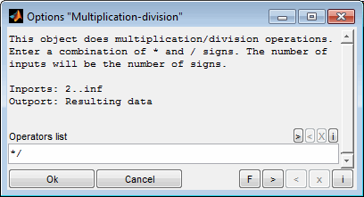
multiplication/division
This object does multiplication/division operations. Enter a combination of * and / signs. The number of inputs will be the number of signs.
Inports: 2..inf
Outport: Resulting data
min/max/mean of multiple inputs
This object does an elementwise minimum/maximum/mean calculation of all inports. Therefore all inport data vectors must have the same dimension and also the outport data will have that dimension.
Inports: 2..inf
Outport: Resulting data
logical operator (AND, OR, NOT)
This object does an elementwise logical operation of the inport data. Therefore all inport data vectors must have the same dimension (or be scalar) and also the outport data will have that dimension. NaN or complex values will be set to NaN in the resulting outport data.
Inports: NOT->1; AND/OR->2..inf
Outport: Resulting data
logical operator bitwise (BITAND, BITOR, BITNOT)
This object does an elementwise bitwise logical operation of the inport data. Therefore all inport data vectors must have the same dimension (or be scalar) and also the outport data will have that dimension. NaN or complex values as well as values >=2^52 will be set to NaN in the resulting outport data.
Inports: BITNOT->1; BITAND/BITOR->2..inf
Outport: Resulting data
getbit
This object gets a single bit out of the input values. Input values are casted to uint64 before. NaN or complex values will be set to NaN in the resulting outport data. "I2" can be used to read the bit nr from inport.
Inport1: Input data
Inport2: Bit nr (if "I2" was configured)
Outport: Resulting data
relational operator (<, <=, ==, >, >=, ~=)
This object does an elementwise relational operation of the inport data. Therefore all inport data vectors must have the same dimension or must be scalar. The outport data will be a vector of same size containing logical zeros and ones. NaN or complex values will be set to false in the resulting outport data.
Inports: 2
Outport: Resulting data
Normalization
This object merges any number of inports to a single channel with a range 0..1. Its main purpose is to create a channel e.g. for stability detection by normalizing all inport channels to the same range, adding them and scaling the result to the range 0 to 1. All inport data vectors must have the same dimension and also the outport data will have that dimension.
Inports: 2..inf
Outport: Resulting data
11.4 Single vector operations (dimensions preserved)
raise to power
This object raises all elements of the inport to a given power value.
The power value can be specified or the expression "I2" can be used to read from inport 2.
Inport1: Input data
Outport: Resulting data
remainder of division (modulo)
This object calculates the remainder after division (modulo).
Two modes are available. In modulo mode the result is either zero or has the same sign as the divisor. In remainder mode the result is either zero or has the same sign as the input data. When the divisor is zero in modulo mode the result will be 0 and in remainder mode it will be NaN.
The divisor value can be specified or the expression "I2" can be used to read from inport 2.
Inport1: Input data
Inport2: Divisor (if "I2" was configured)
Outport: Resulting data
math function (abs, sign, e^, log, 10^, log10, eps, squareroot, accumulated sum/product, NaN? Inf?, ...)
This object does an elementwise math operation of the inport data. Therefore the outport data vector will have the same dimension as the inport.
Inport1: Input data
Outport: Resulting data
trigonometric function (sin, cos, ...)
This object does an elementwise trigonometric operation of the inport data. Therefore the outport data vector will have the same dimension as the inport.
Inport1: Input data
Outport: Resulting data
difference
This object calculates an elementwise difference of the inport data. The difference of a vector decreases its length by one element. You can decide to pad the reduced outport data length with a zeros, ones or NaN. In case the inport data is a matrix the differences will be calculated columnwise.
Inport1: Input data
Outport: Resulting data
sort
This object sorts the inport data and returns the values or their indices. The order can be configured. In case of matrix inport data the sorting can be configured to handle the columns separately or to sort entire rows.
If the option is checked the outport data will contain the indices of the sorted data entries instead of the values. The index numbers are one based. If you for example for sort [0.2 0.1 0.3] the returned indices will be [2 1 3].
Inport1: Input data
Outport: Resulting data or indices
saturation
A saturation object limits its inport to a min. and max. limit. The max. limit is applied last and therefore dominant. The limits can be specified or the expression "I2" / "I3" can be used to read from inports.
Inport1: Input data
Inport2: Lower limit (if "I2" was configured)
Inport3: Upper limit (if "I2"/"I3" was configured)
Outport: Limited output data
in range?
This object indicates whether the inport data is between specified limits. The outport signal will be one if the inport data is between or equal the limits and zero otherwise.
Inport1: Input data
Outport: Resulting data
round
This object does an elementwise round operation of the inport data to an integer value. Therefore the outport data vector will have the same dimension as the inport. NaN or complex values will result in NaN values in the resulting outport data.
Inport1: Input data
Outport: Resulting data
DataType
This object converts the data type of the inport data. Available data types are double, single, uint64, uint32, uint16, uint8, int64, int32, int16, int8 and logical.
Inports: 1
Outport: Resulting data
edge detection
This object detects edges of the inport data. The edge direction and threshold value can be specified or the expression "I2" can be used to read from inport 2.
Inport1: Input data
Inport2: Threshold data (if "I2" was configured)
Outport: Resulting data
S-R Flip Flop
This object implements a S-R Flip Flop with only output Q. The initial value can be configured.
Inport1: "S" set
Inport2: "R" reset
Outport: Resulting data "Q"
fixed step (FixedStep)
This object modifies each value of the inport data to the nearest value divisible by the increment value without remainder regarding an offset. The increment value can be specified or the expression "I2" can be used to read from inport 2.
Inport1: Input data
Inport2: Increment value (if "I2" was configured)
Outport: Resulting data
moving average filter (MovAverage)
This object performs a moving average filter operation. The filter length can be specified and an automatic and guided filtering is also provided.
Inport1: Input data
Inport2: Filter length (if "I2" was configured)
Outport: Resulting data
filter digital FIR
This object performs a digital FIR filter operation.
Inport1: Input data
Inport2: Filter length / Axis data (if "I2" was configured)
Inport3: Filter length (if "I3" was configured)
Outport: Resulting data
PT1 filter
This object performs a PT1 filter operation. The filter factor must be in the range 0 (max. filtering) to 1 (no filtering) or the expression "I" to read from inport 2.
Inport1: Input data
Inport2-4: Filter constant, reset condition, reset value (in that order, depending on "I" configuration)
Outport: Resulting data
outlier removal (OutlierRemoval)
This object performs a outlier removal operation. The criteria can be specified or left empty for automatic detection. A guided operation is also provided.
Inport1: Input data
Outport: Resulting data with outliers set to NaN
counter with reset and limits (count)
This object calculates a cumulated sum. A reset condition and limits are available. To use the counter as an integrator, just multiply the inport data with the difference of its axis.
Inport1: Input data
Inport2-4: Reset condition, reset value, lower, upper limit (in that order, depending on "I" configuration)
Outport: Resulting data
delta limiter (DeltaLimit)
This object performs a hysteresis calculation. The threshold can be entered directly or the expression "I2" or "I3" can be used to read from inport 2 or 3. Note that the "Min. delta" usually is negative.
Inport1: Input data
Inport2: Upper threshold (if "I2" was configured)
Inport3: Lower threshold (if "I3" was configured)
Outport: Resulting data
hysteresis
This object performs a delta (gradient) limitation. The limiting deltas can be entered directly or the expression "I2" or "I3" can be used to read from inport 2 or 3.
Inport1: Input data
Inport2: Max./min. delta (if "I2" was configured)
Inport3: Max./min. delta (if "I3" was configured)
Outport: Resulting data
turn on-off debounce (Debounce)
This object implements a turn on/off debounce. The switching point is recognized when the inport 1 data becomes/leaves the value zero. The delay value can be specified or the expression "I3" can be used to read from inport 3.
Inport1: Input data to debounce
Inport2: Axis data of inport 1
Inport3: Delay data (if "I3" was configured)
Outport: Resulting data
11.5 Vector operations (dimensions changed)
transpose
This object changes the dimensions of a vector or matrix. "transpose" swaps the horizontal and vertical dimension. For a vector is swaps between a column and row vector. "ToColumn" and "ToRow" force a vector direction if the inport data. In the case of a matrix or higher dimensions, a vector is created by arranging all elements one after the other.
Inport1: Input data
Outport: Resulting data
join data
This object joins the data of multiple inports. The direction to join can be specified. "automatic" means that vectors are concatenated in their longer direction. All inports must be vectors having the same direction in this case.
Inports: 2..inf
Outport: Resulting data
remove duplicate (RemoveDuplicate)
This object removes duplicate values from the inport data. In case of matrix inport data the processing is done for each column separately.
Inport1: Input data
Outport: Resulting data
get values by index (GetByIndex)
This object returns a subset of elements of the input data. The values returned are defined by their indices.
Inport1: Input data
Inport2: Indices
Outport: Subset data
set values by index (SetByIndex)
This object modifies a subset of elements of the input data.
The values to modify are defined by their indices. The new values to set at the indexed positions are passed by an inport. So dimensions of the indices and the replacement data must match and the indices must be in the range of the input data dimension.
Inport1: Input data
Inport2: Indices
Inport3: Replacement data
Outport: Modified input data
get column or row (GetColumnRow)
This object extracts one or more columns or rows from the inport data matrix. The index can be specified or the expression "I2" can be used to read from inport 2.
Inport1: Input data
Inport2: Indices scalar or vector (if "I2" was configured)
Inport3: Replacement data
Outport: Resulting columns/rows data
get index (GetIndex)
This object returns a list of all indices of nonzero entries of the inport data. The max. number of indices to return can be limited. The index numbers are one based. So e.g. for the input [2 2 0 0 7] the output will be [1 2 5].
Inport1: Input data
Inport2: Threshold value (if "I2" was configured)
Outport: Resulting list of indices
get threshold index (GetThrsIndex)
This object returns a list of all indices where the inport data crosses a threshold. The threshold value can be specified or the expression "I2" can be used to read from inport 2. Different modes for the crossing direction and order are available.
Inports: 1..2
Outport: Resulting list of indices
11.6 Other operations
statistic of vector
This object calculates a statistical result of the inport data. The result will be a scalar value. The mode to calculate the result can be chosen (e.g. min, max, mean, sum...). In case of matrix inport data the operation will be done column wise.
Some operations lead to an invalid result if some of the inport data is invalid (e.g. NaN or inf). By selecting the “Ignore invalid data” option the operation will ignore invalid data and therefore calculate a valid result even if part of the data is invalid. In case all inport data is invalid the operation will calculate an empty result.
Inport1: Input data
Outport: Resulting data
dimension
This object calculates a dimension of the inport data. The result will be a scalar value.
Inport1: Input data
Outport: Resulting dimension value
struct
This object creates a structure from the inport data using the given field names.
Inport1: Input data
Outport: Resulting structure
11.7 Axes / interpolation
axis of channel (Get X-axis)
This object retrieves the x-axis of a channel from the file or an already existing calculated channel. The axis can be used inside the calculation or connected to an ''Add X-axis'' object to assign the x-axis for this calculated channel. See “Axis objects” for details.
Inports: -
Outport: X-axis data
axis assignment (Set X-axis)
This object is used to assign the X-axis of the calculated channel. If the dimension of the result of the calculation does not match exactly one existing x-axis you have to create an x-axis and assign it to be able to load the calculated data. This object is connected to the x-axis data and does the assignment. To assign an existing x-axis for this calculation use the "Get X-axis" object. See “Axis objects” for details.
Inport1: X-axis data
Outport: -
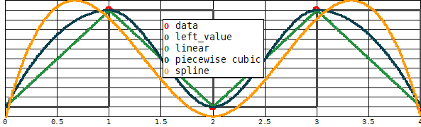
interpolation (channel)
This object does an interpolation of an vector to new axis values. You can select between different interpolation methods.
Left value: The interpolated values are calculated by always selecting the next left (= older) value of the axes points.
Linear: The interpolated values are calculated by linear interpolation of the nearest neighbor axes points.
Piecewise cubic: The interpolated values are calculated by performing a shape preserving piecewise cubic interpolation. There overshoot effect a avoided.
Spline: The interpolated values are calculated by performing a cubic interpolation. Overshoot effects may occur.
The following figure shows the effect of the different interpolation methods.
Inport1: Axis of original data
Inport2: Original data
Inport3: New axis values
Outport: Interpolated data
interpolation (curve)
This object does a curve interpolation. The curve axis and data is passed as inports as well as the new axis values. Different interpolation methods are available.
Inport1: Axis of original data
Inport2: Original data
Inport3: New axis values
Outport: Interpolated data
interpolation (map)
This object does a map interpolation. The map axes and data is passed as inports as well as the new axes values. The calculation is done by linear interpolation. Outside the axes ranges the values are clipped to the last axis breakpoint.
Inport1: Vertical axis of original data matrix
Inport2: Horizontal axis of original data matrix
Inport3: Original data matrix
Inport4: New vertical axis values
Inport5: New horizontal axis values
Outport: Interpolated data
11.8 External interfaces
DCM map/curve/value
This object reads a value, curve or map from a calibration parameter file (DCM, /PaCo, CDF or DCMAT...) and interpolates it to to the corresponding inports or return it.
Parameter type
Choose a parameter type. You can select to load a map, curve, cuboid, cube_4 (or more) or to just use a scalar value.
Mode
Choose the mode to operate. In case of interpolation the parameter will be interpolated to the corresponding inport data. Otherwise the parameter or axis chosen will be returned.
Calibration parameter file
Enter the filename incl. path to use. Leave empty to ask after confirming this dialog or use the following pushbutton to fill this field. Insert "**ask**" or "**ask_once**" to ask the user each time the channel is calculated. In case of "**ask_once**" all objects will share the same file. When a calculation includes DCM objects referencing the same previous file you will be asked whether to transfer the file name to the other objects. This may be done only for the actual or all calculations.
Calibration parameter name
Enter the label name to load. Leave empty to ask after confirming this dialog or use the following pushbutton to fill this field. Insert "**ask**" to ask the user each time the channel is calculated.
Transpose
When selected the horizontal and vertical dimension are swapped. This option must only used with curve and map parameters. When the mode is set to "Interpolation" and the parameter is a map this will lead to interchanging the two inputs. For interpolating curves this will have no effect. For mode "Return*" the parameter or axis horizontal and vertical dimensions will be swapped. So for the axis this means to swap between row and column vector.
This option is normally used to adjust the definition of the x-axis position. While in the SGE Circus, the x-axis is the horizontal axis of a map, in MATLAB/Simulink, for example, it is the vertical axis. In order to use the outport data in a Simulink lookup table, for example, transpose must be used.
Replacement patterns
You can use replacement rules to convert textual parameters to numeric data. Specify one rule per line. These are executed according to the sequence. After this, exactly one number must remain or be created. The string to look for and the numeric scalar replacement value are separated by two colons, like "false :: 0". Alternatively you can use the syntax: "0 -> 'false'”.
The replacement is case insensitive and applied to axes and values. It does not work for parameters with more dimensions than a map.
Examples:
To generate a numeric value 0/1 from false/true string use the following rules.
false :: 0
true :: 1
alternatively:
0 -> 'false'
1 -> 'true'
Inport1: x-axis values (map, curve)
Inport2: y-axis values (map)
Outport: Resulting data
When modifying the file name inside the DCM object and a calculation includes other DCM objects referencing the same previous file you will be asked whether to transfer the file name to the other objects. This may be done only for the actual or all calculations.
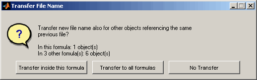
DCM inverse map/curve interpolation
This object reads a curve or map from a calibration parameter file (DCM, PaCo, CDF or DCMAT...) and performs a inverse interpolation to corresponding inports. The file and label name can be specified or "**ask**" can be used to ask the user each time the channel is calculated. In case of "**ask_once**" for the filename all objects will share the same file.
In case of a map you can choose between to do the inverse interpolation in horizontal (x) or vertical (y) direction. In this way, you determine the direction of the inversion. If the inversion is understood as tilting, you decide here the direction of tilting. For a curve inverse interpolation one inport will be created. For a map inverse interpolation two inports will be created. The first one is to connect the values to use for inverse look up. The second one is for the axis values of the dimension not to invert.
For example, if you want to invert a map representing torque (w) over speed (x) and load (y), you have two options:
If you want the result to be a speed, select "x / horizontal direction" and connect a torque signal to the first and a load signal to the second inport.
If you want the result to be a load, select "y / vertical direction" and connect a torque signal to the first and a speed signal to the second inport.
INCA map/curve/value
This object reads a value, curve or map from ETAS INCA software and interpolates it to to the corresponding inports or return it.
Parameter type
Choose a parameter type. You can select to load a map, curve, cuboid, cube_4 (or more) or to just use a scalar value.
Mode
Choose the mode to operate. In case of interpolation the parameter will be interpolated to the corresponding inport data. Otherwise the parameter or axis chosen will be returned.
INCA device name
Enter the name of the INCA device to use. This setting is only necessary in case of labels or variables with the same name on different devices or when an action should take place on an explicit device.
Calibration parameter name
Enter the label name to load. Leave empty to ask after confirming this dialog or use the following pushbutton to fill this field. Insert "**ask**" to ask the user each time the channel is calculated.
Transpose
When selected the horizontal and vertical dimension are swapped. This option must only used with curve and map parameters. When the mode is set to "Interpolation" and the parameter is a map this will lead to interchanging the two inputs. For interpolating curves this will have no effect. For mode "Return*" the parameter or axis horizontal and vertical dimensions will be swapped. So for the axis this means to swap between row and column vector.
This option is normally used to adjust the definition of the x-axis position. While in the SGE Circus, the x-axis is the horizontal axis of a map, in MATLAB/Simulink, for example, it is the vertical axis. In order to use the outport data in a Simulink lookup table, for example, transpose must be used.
Inport1: x-axis values (map, curve)
Inport2: y-axis values (map)
Outport: Resulting data
INCA inverse map/curve interpolation
This object reads a curve or map from ETAS INCA and performs a inverse interpolation to corresponding inports. The INCA device and label name can be specified or "**ask**" can be used to ask the user each time the channel is calculated.
In case of a map you can choose between to do the inverse interpolation in horizontal (x) or vertical (y) direction. In this way, you determine the direction of the inversion. If the inversion is understood as tilting, you decide here the direction of tilting. For a curve inverse interpolation one inport will be created. For a map inverse interpolation two inports will be created. The first one is to connect the values to use for inverse look up. The second one is for the axis values of the dimension not to invert.
For example, if you want to invert a map representing torque (w) over speed (x) and load (y), you have two options:
Inport1: map values to invert (map, curve)
Inport2: axis values (map)
Outport: Resulting inverse axis data
When modifying the file name inside the DCM object and a calculation includes other DCM objects referencing the same previous file you will be asked whether to transfer the file name to the other objects. This may be done only for the actual or all calculations.
If you want the result to be a speed, select "x / horizontal direction" and connect a torque signal to the first and a load signal to the second inport.
If you want the result to be a load, select "y / vertical direction" and connect a torque signal to the first and a speed signal to the second inport.
Simulink simulation
This object performs a Simulink simulation. Data exchange is done using MATLAB COM Automation server. The inport data of the object is first written to the MATLAB workspace. Then the simulation is started and after termination the output is retrieved. See “Simulink simulation“ for details.
Inport1..n: Inport values to transfer to Simulink
Outport: Resulting data from Simulink
Simulink DLL
This object computes the output of a Simulink Host-Based Shared Library (*.dll) created with the "ert_shrlib.tlc" build target. It is possible to access signals and parameters to set them to values produced by CalcGuide and to retrieve the simulation result. See “Simulink Host-Based Shared Library (*.dll)“ for details.
Inport1..n: Inport values
Outport: Resulting data
Inport1: map values to invert (map, curve)
Inport2: axis values (map)
Outport: Resulting inverse axis data
When modifying the file name inside the DLL object and a calculation includes other DLL objects referencing the same previous file you will be asked whether to transfer the file name to the other objects. This may be done only for the actual or all calculations.
MATLAB function / mex
TThis object performs a MATLAB function or mex call. Data exchange is done using MATLAB COM Automation server. The inport data of the object is first written to the MATLAB workspace. Then the calculation is performed anf the output is retrieved.. See “MATLAB function / mex“ for details.
Inport1..n: Inport values to transfer to MATLAB
Outport: Resulting data from MATLAB
11.9 Miscellaneous
if/else switch
This object switches between two inputs. If the switch condition is a scalar value, the whole input data vectors/matrices are switched. If the switch condition dimension matches the input data dimensions, the switch operation is done elementwise. If the switch condition is true, the first input data is chosen, otherwise the second.
Inport1: Switch condition
Inport2: First data inport
Inport3: Second data inport
Outport: Output data
subsystem
Subsystems are used to structure extensive calculations or to reuse parts of calculations as they can be copied easily. Subsystems additionally have inport objects. These make available the data from the lines connected outside the subsystem. Similarly they have outports. A subsystem must have exactly one outport object.
Inports: 0..inf
Outport: Resulting data
for loop subsystem
For loop subsystems can be used to implement iterative calculations. They have three additional inports for the start, increment and final value of the loop counter. Inside the subsystem a LoopCnt object is available to access the loop counter. A for loop will show up a waitbar if is is executed.
Remember that by default all calculations are performed vector based in one step. So for example to calculate a cumulated sum there is no need to use a for loop subsystem – see section ”Vector based calculation strategy“ for details.
Inport1: loop counter start value
Inport2: loop counter increment value
Inport3: loop counter final value
Inport4..inf: inports
Outport: Resulting data
comment object
This object is used to display a static text. It has no influence to the calculation. Empty spaces at the beginning and end will be removed. If you want to increase the size of the block use a point or any character before and after the spaces.
Inports: -
Outport: -
line branch
A line branch is used to split data lines or to create bends in a line to avoid elements crossed by lines.
Inport1: Input data
Outport: Identical to inport data
visualize
This object performs a visualization of the inport data when the calculation is executed. It has no influence to the calculation and can be used for debugging purposes. Visualization objects are not regarded when performing a test calculation if not explicitly enabled in the configuration object.
Inport1: Input data
Outport: Identical to inport data
test calculation skip
If this object is included the test calculation will be skipped and the channel is calculated immediately using the actual data. Use it to avoid warnings caused by the special test data.
Inports: -
Outport: -
12 Present, print, organize
12.1 Copy to clipboard, print
The CalcGuide makes it available to export the actual view into the clipboard or file formatted in a way that is suitable to be useful for different targets (Ctrl + shift + c).
Document
Email
File
Printer
This can be different sizes of clipboard content. "Email" and "Document" are specially sized to fit into a email or document software. "Email" creates a bitmap format while "Document" creates a vector format. Some paper formats are also available and all windows can be printed and saved to file in various formats.
The created window is configurable. So you can move objects. It is also possible to add lines, arrows, text boxes etc. to the window to explain or highlight.
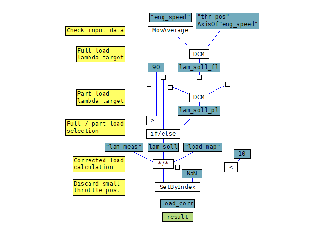
During creation some options will be asked to define the base layout of the window.
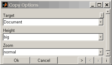
After closing the window the content will be copied to clipboard and can be pasted / used in the target software.
12.2 Window handling
Since the SGE Circus offers to open a considerable number of windows an automatic window handling feature is implemented. Using the corresponding menu item enables to arrange all or a subset of the windows of the current session.
Close windows
This feature enables to close visible and invisible windows automatically.
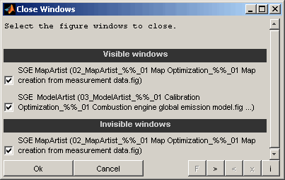
Windows
Select which windows to close. The windows will be closed without saving anything and without any further confirmation. Visible and invisible windows will be listed separately.
Resize windows
This feature enables to automatically set windows to fixed sizes or to maximize, minimize and restore them.
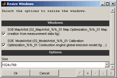
Windows
Select which windows to resize.
Size
Select the desired window size. It is possible to maximize, minimize and restore windows. Additionally a set of fixed standard sizes are available.
Arrange windows
This feature enables to automatically arrange windows.
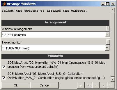
Window arrangement
Select the layout of the arrangement. It is possible to maximize, minimize, restore or close all selected windows. Additionally column and row based layouts are available.
Example: "2-3 of 5 rows" means that the screen is split into 5 rows and the second and third row is used for the layout.
Target monitor
Select the target monitor for the windows to arrange in case of multiple monitors are connected to the computer.
Windows
Select which windows to include into the arrangement.
Toggle windows periodically
This feature enables to automatically toggle windows to create kind of a movie. This can be used to compare windows.
Cycle time
Select the the time to wait before activating the next window.
Maximize windows
If enabled the windows will be maximized before toggle to ensure identical size.
Windows
Select which windows to toggle periodically.
13 General information
Duplication, processing, distribution or any form of commercialization of the documents content beyond the scope of the copyright law shall require the prior written consent of the SGE Ingenieur GmbH. All trade and product names given in this document may also be legally protected even without special labeling (e.g. as a trademark).
MATLAB, Simulink and Stateflow are registered trademarks of The MathWorks Inc., Natick, MA, USA.
The SGE Circus includes Third Party Software. For details please refer to the → SGE Circus documentation.
SGE Ingenieur GmbH – www.sge-ing.de
Copyright 2011-